From Clicks to Conversions: Building a Stacked Regressor for the Engage 2 Value Kaggle Competition

Final score: R² = 0.69272, ranked 125 on the Kaggle leaderboard.

Most analytics dashboards present a comforting illusion: clean charts, neat funnels, percentages that round to whole numbers. The underlying data, of course, rarely cooperates. The Kaggle competition engage-2-value-from-clicks-to-conversions is a fairly honest reminder of that. You are handed 116,023 anonymised web sessions, fifty-two columns of mixed device, geo and traffic metadata, and a single regression target — purchaseValue — that for the overwhelming majority of sessions is exactly zero. Your job is to predict, for each session in a held-out set, how much money that visitor will generate.

This post walks through how I approached the problem, what the data actually looks like once you stop trusting the column names, which feature engineering ideas paid off, why I ended up with a stacked ensemble rather than a single boosted tree, and where the model still leaves performance on the table.

The shape of the problem

Predicting purchase value from clickstream data is a classic zero-inflated, heavy-tailed regression task. A huge fraction of visitors look at a single page and bounce, contributing nothing. A vanishingly small fraction of visitors place orders, and a tinier fraction still place very large orders that dominate the loss function. The training set bears this out almost comically: the 25th, 50th and 75th percentiles of purchaseValue are all zero, while the maximum is 2.31 × 10¹⁰.

The target distribution. The single visible bin near zero contains the bulk of all 116k sessions; everything to the right is a thin tail of high-value purchases.

The implication is immediate. A linear model with mean-squared error will be dragged around by the outliers. A model that predicts the global mean will score zero R². And any feature transformation that ignores the skew will leak signal. So the choice of model family — tree ensembles, with a regularised linear meta-learner sitting on top — is essentially decided by the histogram above before a single line of modelling code is written.

What the columns actually contain

The competition data is the public Google Analytics demo export, and that origin shows up in the schema. Out of 52 columns, a striking number are placeholders or near-constants:

• Thirteen columns are literally the string "not available in demo dataset" for every single row (device.screenResolution, device.flashVersion, device.browserVersion, browserMajor, geoNetwork.networkLocation, and friends).

• totals.visits is always 1. totals.bounces is always 1 when it is present at all. locationZone is always 8. screenSize is always "medium". socialEngagementType is always "Not Socially Engaged".

• Several columns are heavily missing: trafficSource.adContent has only 3% non-null values, the four trafficSource.adwordsClickInfo.* columns sit around 4%, trafficSource.referralPath is 37% present, and new_visits is 69%.

This is genuinely useful information. It tells me to lean on the columns that do vary — and there are plenty:

Feature	Cardinality	Dominant levels
browser	34	Chrome 73 %, Safari 17 %, Firefox 3 %
os	18	Windows 34 %, Macintosh 32 %, Android 14 %, iOS 11 %
deviceType	3	desktop 75 %, mobile 22 %, tablet 3 %
userChannel	8	Organic 40 %, Referral 19 %, Social 18 %, Direct 16 %
geoNetwork.continent	6	Americas 60 %, Asia 19 %, Europe 17 %
locationCountry	193	United States 52 %, India 5 %, UK 3 %
geoNetwork.region	388	California 16 %, New York 5 % (52 % unavailable)
trafficSource	161	google 38 %, (direct) 32 %, youtube.com 17 %

The high-cardinality features here (trafficSource, geoNetwork.region, geoNetwork.city, trafficSource.referralPath) are exactly the ones that will need careful encoding later — one-hot would explode the feature space, and an ordinal encoder would invent a fake ordering. Target encoding is the natural fit.

 Numeric features at a glance. The mix of uniform (userId), near-constant (totals.visits), strongly right-tailed (sessionNumber) and temporally spread (sessionId) distributions tells us we will need log transforms, per-user normalisation, and at least some time-derived features.

A pairplot of the top numerically-correlated features with the target makes the non-linearity even clearer: high-purchaseValue sessions cluster at moderate pageViews and sessionNumber values, not at the extremes. There is no straight line through this point cloud that is going to do good work.

Pairwise relationships with purchaseValue. The off-diagonal scatter plots show clearly non-linear, clustered structure — a strong argument for tree-based learners over plain linear regression.

The system

Architecturally the project is intentionally simple. Everything lives in a single Jupyter notebook that runs either on Kaggle's hosted notebooks or on a local Python environment with the same set of libraries (pandas, numpy, scikit-learn, xgboost, category_encoders, kagglehub). There is no separate training service, no model registry, no orchestration layer — just an end-to-end script that reads the CSVs, builds features, fits the model, and writes a submission file.

High-level system architecture. The Kaggle competition data is pulled with kagglehub, the notebook does all the work in-process, and the trained Stacking Regressor writes a single submission.csv.

That simplicity is deliberate. For a Kaggle competition the marginal value of building infrastructure is essentially zero; what matters is iteration speed on features and models, and a single notebook makes that as fast as it can be.

The pipeline, end-to-end

The full pipeline. Three candidate model families are tuned in parallel; the Stacking Regressor wins on validation R², gets refit on the full training set, and produces the final submission.

The flow is roughly:

1. Authenticate and download the competition data through kagglehub.

2. Explore: schema, descriptive stats, target distribution, numeric distributions, pairwise relationships.

3. Impute: numeric NaNs get the median, categorical NaNs get the most-frequent value. This is intentionally crude — the heavy lifting happens later.

4. Engineer features: roughly forty new columns, organised into eight families (see below).

5. Target-encode every categorical column with category_encoders.TargetEncoder, which replaces each level with the mean of purchaseValue for that level (with smoothing).

6. Select features via RFE on top of an XGBRegressor, keeping the top eighteen.

7. Train and validate three candidates: ElasticNet, HistGradientBoostingRegressor, and a Stacking Regressor.

8. Refit the best model (the Stacking Regressor) on the full training set and predict on the test set, producing submission.csv.

The order matters. RFE has to come after target encoding (or the selector will see categorical columns it cannot evaluate), and the imputer has to come before feature engineering (or the engineered features inherit NaNs from their inputs).

Feature engineering: where most of the gain came from

If a Kaggle ranking is decided by a small number of decisions, this is the section where almost all of them happened.

Eight families of engineered features. Everything flows through target encoding and then through Recursive Feature Elimination, which keeps only the eighteen most predictive columns.

I grouped the new columns by purpose, because that made it easier to add and ablate them as a unit:

• Target-mean encodings — city_avg_spend, region_avg_spend, device_avg_spend. These inject a strong historical prior: how much do visitors from a particular city / region / device type usually spend.

• Engagement metrics — engagement = totalHits + pageViews - bounces, is_bounce, bounce_ratio, bounce_per_visit, bounce_per_hit, bounce_rate_x_page. These compress "how active was this session" into a small number of correlated columns.

• Ratios and interactions — hits_per_page, visit_per_session, hits_x_visits, engagement_x_city_avg, hits_x_hour and friends. Multiplications and divisions of columns that, individually, the model could in principle reconstruct, but in practice rarely does.

• Log transforms — log_totalHits, log_pageViews, log_totals.visits, log_hits_x_visits. Right-skewed numerics get tamed with log1p.

• Time features — hour, weekday, is_weekend, and a categorical hour_bin (Night / Morning / Afternoon / Evening) derived from sessionStart.

• Combo categoricals — channel_device, device_region_combo, channel_x_region. These cross-products capture interactions that a single tree split can't easily learn from the raw columns alone.

• User-level aggregates — user_avg_hits and a per-user z-score z_hits. This is where the data leaves "session-level features" and starts using "this user's baseline" as context.

• Frequency encodings — geoNetwork.city_freq, geoNetwork.region_freq. Popular cities and regions get a higher weight than rare ones.

Once every categorical column (raw and combo) is target-encoded, the table has nearly seventy columns. RFE on top of an XGBoost base estimator then trims it down to the eighteen most predictive features — small enough that the downstream stacking model trains in a reasonable amount of time, large enough to retain the most informative signal.

The model: a stacked ensemble, not a boosted tree

A natural reaction to "skewed regression on tabular data" is "just use XGBoost". Several iterations in, I had tuned XGBoost reasonably well and the validation R² was still leaving signal on the table. The issue was that XGBoost on its own was confident about the head of the distribution (zero-revenue sessions) but volatile on the tail — and the tail is where the loss actually comes from.

Stacking is a fairly heavy hammer for this, but it solved the right problem. The level-0 base learners are a tuned Random Forest and a tuned XGBoost regressor; the level-1 meta-learner is a Pipeline of StandardScaler followed by a strongly-regularised Ridge(alpha=100). The meta-learner sees both the out-of-fold predictions of the base models and the original eighteen features (because passthrough=True), which lets it learn a small correction on top of the ensemble.

The stacking regressor. The two base learners are deliberately diverse — one bagged, one boosted — so that their errors are not too correlated; the Ridge meta-learner blends them and can also lean directly on the original features through the passthrough connection.

The sklearn set_config(display='diagram') render of the actual fitted estimator looks like this:

The same model, rendered automatically by scikit-learn from the fitted pipeline object.

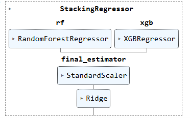
Two specific choices are worth calling out:

1. passthrough=True. Without it, the Ridge meta-learner only sees two numbers per row (the two base predictions) and has very little flexibility. With it, the meta-learner can recover information that the base learners discarded — at the cost of higher variance, which is exactly why the Ridge regularisation is strong (alpha=100).

2. bootstrap=False on the Random Forest. Combined with max_features='log2', this trades some of the variance reduction that bagging usually provides for a tighter fit per tree, which the stacking layer can then de-correlate.

For comparison, I also tuned an ElasticNet pipeline (StandardScaler → ElasticNet, RandomizedSearchCV over fifty values of alpha and twenty of l1_ratio) and a HistGradientBoostingRegressor (small grid over max_iter, max_depth, learning_rate, max_leaf_nodes). The ElasticNet model was the floor — competitive only because of the engineered features doing the heavy lifting — and HistGradientBoosting was a close second to the stacking model. I kept them in the notebook because they are useful sanity checks: if your stacking model is not beating a tuned single-learner baseline, something is wrong with either your feature pipeline or your stack.

Results and ranking

The final Stacking Regressor scored R² = 0.69272 on the competition's hidden test set and placed 125 on the leaderboard. For a tabular regression task with a hard zero-inflated tail, an R² in the high 0.6s suggests the model is genuinely capturing the head of the distribution well, while the tail — those rare, very large purchases — remains the dominant source of remaining error.

A few honest observations about where the remaining performance is:

• The top of the leaderboard is, in my reading, almost certainly a mix of more aggressive target transformations (log-transforming purchaseValue and predicting that, then inverting), more careful cross-validation schemes that respect the user-level grouping, and models like CatBoost / LightGBM that handle high-cardinality categoricals natively.

• My target encoding is a single global pass over the training set; doing it inside a K-fold loop would reduce target leakage and is one of the highest-leverage changes I would make next.

• The constant placeholder columns are currently kept and target-encoded along with everything else. Dropping them earlier would not change performance, but it would shorten the encoder's fit time noticeably.

  
  

Takeaways

If this project has a thesis, it is that on tabular regression problems with messy real-world data, the feature engineering is the model. The choice between Random Forest and XGBoost matters; the choice between a single boosted tree and a small stack matters less than expected; and neither of those decisions is anywhere near as important as deciding to log-transform skewed columns, to target-encode the high-cardinality categoricals, and to add a handful of cross-products and aggregates that encode the actual semantics of the data.

The stacking model is the right hammer for the last few points of R², but it sits on top of a feature table that is already doing most of the work. A small Ridge regression on the same eighteen features would not score 0.69, but it would score embarrassingly close — which is, I think, a healthy reminder that exotic model architectures rarely rescue weak features, while strong features keep simple models competitive.

For anyone tackling a similar competition: start with the histograms, spend most of your iteration budget on the engineered columns, and only reach for stacking once you have a single-model baseline you trust.